As is often true with intellectual property work, I am unable to share the algorithm or go in depth about the method of storage.
That being said, the algorithm is probabilistic, employs a coarse-to-fine search, and is mathematically unrelated to other common image compression methods, such as DCT.
Mathematical behavior
Computational cost and reconstruction quality
Two parameters control the compression process: the quality parameter q and the search depth d. The relationships below describe their effect for a fixed input image and encoding configuration, with q > 0 and integer d ≥ 1.
q
Quality parameter
d
Search depth
T
Encoding time
S
Compressed file size
Time complexity
The algorithm has time complexity O(q · d): the quality parameter multiplied by search depth. The work model grows linearly with either parameter when the other is held fixed.
Using q · d as a work model, doubling either parameter doubles the modeled work; doubling both multiplies it by four. These factors describe the model, rather than exact measured runtimes.
Storage grows linearly with q
The compressed image payload is proportional to q. Allowing for fixed file overhead gives the model below, where S0 is the overhead and cS is the storage cost per unit of q.
Doubling q doubles the variable payload. Search depth controls encoding effort without increasing storage in this model. This describes the compressed file on disk, not the working memory needed by the encoder.
Power-law convergence with search depth
Let E(q, d) denote reconstruction error, measured here by mean squared error (MSE) between original and reconstructed pixel values: smaller error means greater fidelity. Because the search is probabilistic, the relationship describes its average behavior rather than a guarantee for each individual run.
A model of the stated convergence is a residual error floor plus a term that decays as a power of search depth:
Here E∞(q) is the error floor at a fixed q, A(q) ≥ 0 controls the remaining search error, and α > 0 is the convergence exponent. These quantities depend on the image and measurement setup; the depth benchmark below gives a numerical fit at q = 100.
At fixed q, deeper search brings the reconstruction closer to a constant error floor. Doubling d reduces the excess error above that floor by a factor of 2−α in this model. This floor concerns increasing depth while holding q fixed.
Inverse power-law error with q
At a fixed depth d0, increasing q reduces MSE according to an inverse power law with no additive error floor. For the measurements at d0 = 100,000, the supplied exponent is β = 0.29:
B(d0) > 0 is a scale factor for the fixed depth and image. The model tends toward zero error as q increases, rather than a positive constant; the finite measurements below support the trend over the tested range.
Doubling q multiplies modeled MSE by 2−0.29 ≈ 0.818, a reduction of about 18.2%, while doubling the variable payload and modeled encoding work. A reciprocal-error quality proxy, Q = 1/E, therefore scales as q0.29 at this depth, rather than linearly. This proxy is distinct from PSNR and from a perceptual quality score.
Measured performance
Benchmark results
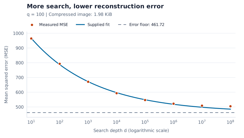
At q = 100, the compressed image occupies 1.98 KiB and achieves higher PSNR than a 4.22 KiB JPEG in this comparison. That is approximately 53.1% less storage. The measurements below show how mean squared error (MSE) changes with search depth while q and compressed file size stay fixed.
Search depth versus pixel error
The fitted relationship uses d for search depth, matching the notation above:
The model approaches an MSE of 461.72 as depth increases. Each tenfold increase in d multiplies the modeled excess error above that floor by 10−0.1904 ≈ 0.645, a reduction of about 35.5%, while multiplying the work model by ten.
Dots show measurements; the solid curve shows the supplied fit. Search depth uses a logarithmic axis: each tick represents ten times as much search. The dashed line marks the modeled error floor.View all eight measurements
Measured MSE at q = 100 and a file size of 1.98 KiB
Search depth (d)
MSE
10
964.23
100
792.66
1,000
670.66
10,000
593.07
100,000
546.73
1,000,000
522.1648
10,000,000
508.65
100,000,000
504.616
Quality parameter versus pixel error
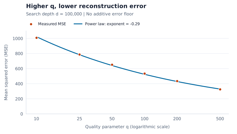
Holding d = 100,000 fixed, the six measurements below vary q from 10 to 500. MSE decreases from 1007.43 to 324.4451 as the quality parameter increases.
The curve keeps the supplied exponent of 0.29 and has no additive constant. Its scale coefficient is estimated from all six points by least squares on MSE, with the exponent held fixed.
Dots show measurements at fixed depth; the solid curve shows the inverse power-law model. The quality parameter uses a logarithmic axis. This model has no positive error floor.View all six measurements
Measured MSE at search depth d = 100,000
Quality parameter (q)
MSE
10
1007.43
25
786.03
50
651.01
100
533.6056
200
434.1
500
324.4451
Broader benchmark summary
Across the full Kodak PhotoCD benchmark at q = 200 and d = 10,000,000, the algorithm achieves lower average MSE and higher average PSNR than JPEG, while using about 6.2% less storage.
Full-benchmark averages at q = 200, d = 10,000,000
Metric
Algorithm
JPEG
File size
3.96 KiB
4.22 KiB
MSE ↓
408.9
482.9
PSNR ↑
22.86 dB
21.48 dB
At q = 100, as shown earlier, the algorithm still outperforms JPEG at 1.98 KiB versus 4.22 KiB—approximately 53% smaller. That benchmark achieved mean 500:1 compression at 22.2 dB PSNR. The algorithm’s advantage over JPEG wanes as file size increases, making it primarily suitable for compression at very small file sizes.
See the difference
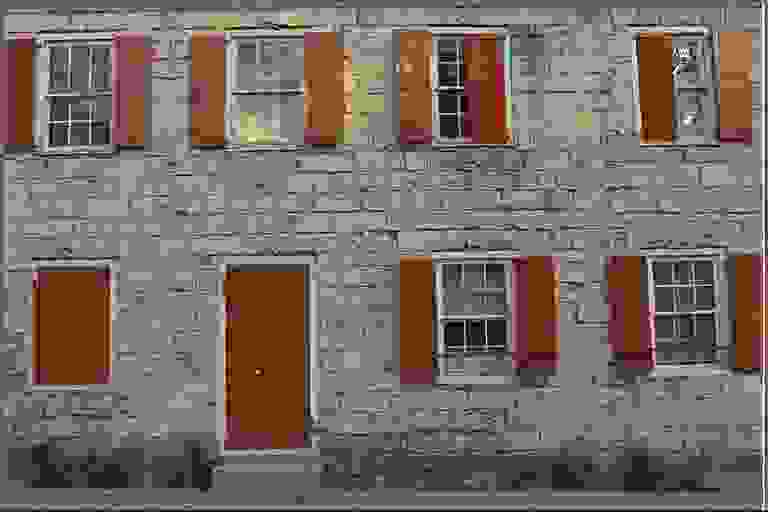
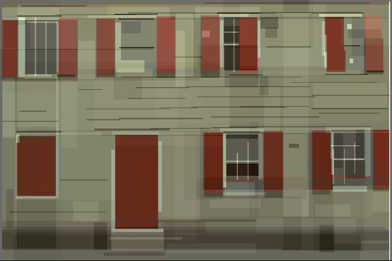
Explore four examples at q = 200, d = 10,000,000, alongside their originals and JPEG counterparts. Each algorithm output has an encoded size of 3.96 KiB. The per-image measurements below are separate from the full-benchmark averages above.
AlgorithmJPEG
50% / 50%
Drag across the image or use the slider to compare the same pixels. Use the arrow keys on the slider for precise control; Home and End reveal either image in full.
MSE and PSNR are calculated from the displayed previews against each original, averaging squared differences across RGB channels with an 8-bit peak of 255. Lower MSE and higher PSNR indicate closer pixel reconstruction. Algorithm previews are JPEG exports for viewing; their download sizes do not represent the reported 3.96 KiB encoded payload. JPEG sizes are measured from the supplied files and vary by image.